Utility: Sub-model

Description

Generates a sub-model from a global model.

A sub-model is a part of the global model that can be analysed independently of the global model whilst producing results that match the global modal. It typically comprises selected elements and their attributes, load cases and freedom cases, with the addition of boundary attributes to enforce the results of the global model at the sub-model boundary.

To apply the boundary attributes, the sub-model must be generated while a result file is open. If it is generated while no result file is open, the sub-model will still be produced, but without boundary attributes. This can still be useful for the purpose of extracting a part of the global model as a separate file, but generally it cannot be run to match the global model results.

If a result file is open when the sub-model is created, additional boundary conditions (attributes) are applied to the boundary nodes of the sub-model. The type of boundary conditions applied depends on the type of result file. For heat transfer analysis, the boundary nodes are assigned fixed node temperature attributes. For the structural solvers, the boundary nodes are assigned enforced displacement and rotation attributes.

Sub-models can be generated for any result file, but not all result files will produce sub-models that represent a physically meaningful situation, or produce a file that can be run independently to duplicate the global model results.

The most common solver types for physically meaningful sub-models are the steady-state heat transfer solver, the linear static solver and the nonlinear static solver. The time-dependent solvers (i.e., transient heat solver, quasi-static solver, linear and nonlinear transient dynamic solvers) will produce meaningful sub-models in that they represent a correct snapshot at the relevant time step. However, additional setup work is required before those sub-models can be run to reproduce the global model results. Sub-models produced from the other solvers (i.e., linear buckling, load influence, natural frequency, harmonic response and spectral response) will usually not be of practical value.

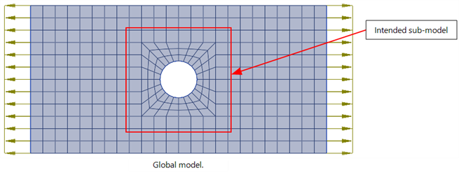
The following sequence of image illustrates a typical linear static sub-modelling workflow.

A global model is generated. Usually the region to be sub-modelled is identified at this stage so that an appropriate meshing strategy can be adopted.

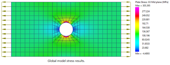
An analysis is run and results are inspected.

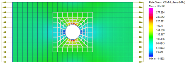
The set of elements to be sub-modelled is selected and the sub-model utility is executed. This saves the selected elements into a new Strand7 file.

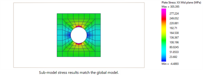
This file can be opened and solved to ensure that it produces the same results as the global model (the grey global model boundary outline below is drawn only for clarity, it is not part of the sub-model).

If the sub-model is re-meshed by subdividing (Mesh Tools: Subdivide), a refined model is produced with the enforced boundary conditions linearly interpolated on the new boundary nodes produced by the subdivision. This enables a more efficient mesh convergence study to be undertaken compared with refining the global model.

Steady Heat Solver

A sub-model from a linear steady heat analysis produces a model that can itself be run using the steady heat solver to produce identical results to the global model. For a nonlinear steady heat analysis, the sub-model results will typically match the global model results closely, if not exactly.

Linear Static Solver

A sub-model from a linear static analysis produces a model that can itself be run using the linear static solver to produce identical results to the global model. The sub-model will contain one new load/freedom case pair for each result case in the global model. The new freedom cases will contain the total enforced displacements and rotations from each result case in the global model.

Nonlinear Static Solver

A sub-model from a nonlinear static analysis produces a model that can itself be run using the nonlinear static solver to produce identical results to the global model. The nonlinear solver will be automatically set up to solve the sub-model using a staged analysis, irrespective of whether the global model used a staged analysis or not. There will be one stage for each result case in the global model, with one new freedom case for each stage. The new freedom cases contain the incremental displacements and rotations from stage to stage.

Running this newly created staged analysis in the sub-model will produce identical results to the global model.

Node vs Element Results

The nodal temperature results of heat transfer sub-models will match the nodal temperatures of the global model. Similarly, the nodal displacement results of the sub-model will match the nodal displacements of the global model.

Element results extracted at the element centroid and Gauss points will also match between sub-model and global model.

Extrapolated and averaged element-based nodal results (e.g., stress or flux) in the sub-model will match the global model at nodes that are not on the boundary of the sub-model. Nodes that are on the boundary will generally produce slightly different results because, in the sub-model they are not being averaged with the same elements as in the global model.

Common Uses

Critical areas that require further investigation or mesh refinement are usually identified after solving the global model. These areas of interest can be selected for sub-model creation and then subjected to mesh refinement. Solving the locally refined sub-model provides further insights into those critical areas without modifications to the global model.