SOLVERS: Load (Nonlinear Transient Dynamic)

Description

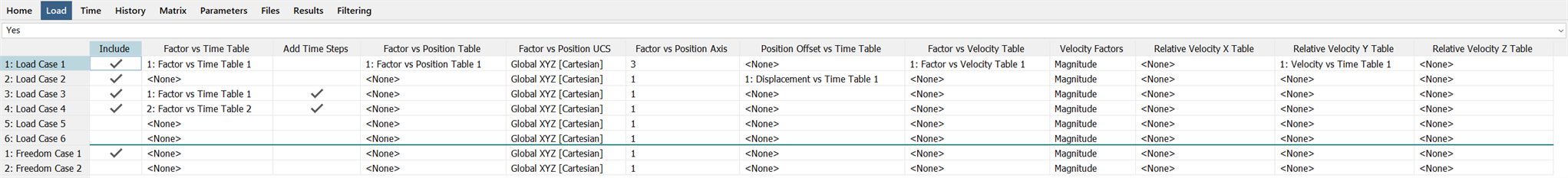
Selects the load and freedom cases to include in the Nonlinear Transient Dynamic solver, and assigns Factor vs Time tables, Factor vs Position tables and Factor vs Velocity tables for each load and/or freedom case. All included cases are combined and act simultaneously.

If a case is excluded (i.e., not checked), it makes no contribution to the solution.

If a case is included (i.e, checked), its contribution depends on the tables assigned to it. If no tables are assigned to an included case, its unscaled loads are always added to the solution.

The factor at a particular time step for an included case is determined from the product of factors due to the vs time, vs position and vs velocity tables.

Factor vs Time Table and Add Time Steps

This applies to both load cases and freedom cases.

The factor at a particular time step for an included case is determined from the vs time table. If a table is not specified (i.e., <None> is selected), a factor of 1.0 is used. If a table is specified, the factor is calculated by interpolating the table data at each time step of the analysis. If the time instance at any time step is outside the range of the table, the factor is set to zero.

When applied to freedom cases, the factor scales the enforced displacement values at nodes. If restraints at nodes are all zero values (i.e., only fixed restraints are included), the factor has no effect.

If a Factor vs Time table is selected and Add Time Steps is set, additional time steps may be inserted automatically by the solver. These additional time steps correspond to data points (time values) in the Factor vs Time table that occur within the solution time range specified for the analysis (SOLVERS: Time Steps). Furthermore, if Save table-inserted steps is set (SOLVERS: Time Steps), those additional time steps are saved to the result file.

Factor vs Position Table, Factor vs Position UCS, Factor vs Position Axis and Position Offset vs Time Table

This applies only to load cases, not to freedom cases.

These tables with corresponding UCS and axis settings can be used to scale the load applied to a node based on the position of the node at any time step. During the analysis, the current position of a node is transformed to the selected Factor vs Position UCS. The corresponding ordinate specified by the Factor vs Position Axis is then used as the x axis on the selected Factor vs Position Table to calculate a factor by interpolation. This factor scales the external load applied to the node. An example of the use of this feature is the modelling of a floating ship - here the pressure at any point on the hull depends on the position of the hull with respect to the water line (i.e., its depth).

If the selected ordinate of a node exceeds the range of the Factor vs Position table, the table is extended by maintaining the first or last y value. Therefore, the position factor will be equal to the first or last value in the table, depending on which end of the table has been exceeded.

To provide more flexibility, the effective position of the specified ordinate of the node can also be offset as a function of time. This is achieved by assigning another table to the load case, the Position Offset vs Time Table. If assigned, this table will apply a position offset to the specified ordinate of the node as a function of time. This offset position, rather than the true position of the node, is then used to look up the Factor vs Position Table. An example of the use of this feature is the modelling of the filling of a tank with fluid. A Factor vs Position table can be defined to represent a hydrostatic pressure distribution, and the tank can then be effectively moved up and down, relative to the pressure distribution, by the use of the Position Offset vs Time Table. Note that this movement is a virtual movement. It does not generate any inertia or momentum in the structure.

Factor vs Velocity Table, Velocity Factors and Relative Velocity Tables

This applies only to load cases, not to freedom cases.

If a Factor vs Velocity table is selected, the applied load is scaled based on the current velocity of the node on which the load is applied. An example is the drag force of a moving object - the drag force increases as the object accelerates through a fluid medium.

Velocity Factors = Components

The components of the applied load in the three global directions are independently scaled by the load factors in the respective vs Velocity tables based on the velocity components. Both positive and negative velocities can be used in the vs Velocity table; a negative velocity component refers to node movement in the minus direction of the axis.
Velocity Factors = Magnitude

The load is scaled based on the dot product of the direction of the load (normalised) and the velocity vector. This produces a single velocity value with which the vs Velocity table is interpolated.

If the object is stationary while the fluid medium moves around it instead (e.g., wind blowing around a sign post), Velocity vs Time tables can be specified under the Relative Velocity X, Y and Z tables to define the velocity of the fluid medium relative to the object. If the fluid medium has a positive relative velocity, it means that the object has a negative velocity when compared to the fluid medium.