SOLVERS: Matrix
Description
Selects and configures the stiffness matrix solution scheme for the analysis.
MATRIX SCHEME
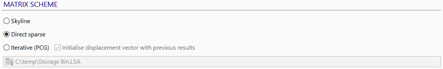
Skyline
The Skyline scheme is efficient for small models and for large brick models consisting of regular meshes. The bandwidth of the matrix is the most significant parameter affecting the performance of this option.
The Skyline option is available for all solver types.
Direct Sparse
The Direct Sparse scheme is a high performance option that is useful for medium to large models. Sparse solvers allow very fast solution of large systems of equations by exploiting the so-called sparsity of the matrix. A matrix is sparse if the number of non-zero entries is small compared with the total number of entries in the matrix.
Most large FE models generate sparse matrices — typically the initial non-zero terms make up less than 10% of the banded matrix. However, as decomposition of the matrix proceeds, many of the terms that were initially zero become non-zero, thereby "filling in" the zeros in the matrix. By ordering the nodes in the matrix in a certain way, it is possible to reduce this fill-in. Consequently, terms that start off as zero and remain zero after the decomposition, need not be acted upon during the process nor do they need to be stored.
It is not possible to find an ordering that minimises this fill-in without actually checking every possible node combination. However, there are algorithms that find orderings that approximately minimise the fill-in. The algorithm used for the direct sparse solver in Strand7 is known as AMD (Approximate Minimum Degree).
This Direct Sparse option is available for all solver types.
Iterative (PCG)
The Iterative scheme is mostly useful for very large models, particularly large brick models. This solver requires significantly less storage than the other solvers because the stiffness matrix is not actually decomposed; only the initial non-zero terms are stored and processed. The solution is found by iteration using the so-called Pre-Conditioned Conjugate Gradient algorithm, minimising the residual between the applied loads and the effective loads (which are equal to the matrix multiplied by the current displacement vector estimate). This option performs best when the global stiffness matrix is well-conditioned (i.e., it has a low condition number). This is usually the case for 3D brick and 2D elasticity problems, but less so for structures containing thin shells.
The Iterative (PCG) scheme is available for the following solve types: Linear Static, Nonlinear Static, Load Influence, Quasi-static and Steady State Heat. For mode superposition solvers (Harmonic Response, Spectral Response, Linear Transient Dynamic) this solver is not relevant because no matrix reduction is performed. For all other solvers, this scheme is not available.
-
Initial
If set, selects a previous solution file as the initial estimate of the solution.
In situations where there are multiple load cases, and only some of the loads have been changed between different versions of a model, the calculation will be much faster by using this option since the cases that have not changed will converge right away.
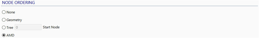
NODE ORDERING
Node ordering aims to reduce either the size of the matrix, the bandwidth or the fill-in during the decomposition of the global stiffness matrix, to improve the performance of the various solver schemes described above. Note that node ordering only renumbers the nodes internally for the solver, it does not affect the user-defined node numbers.
For the Skyline scheme, either Geometry or Tree will provide the best performance.
For the Direct Sparse scheme, the AMD option almost always offers the best performance.
For the Iterative (PCG) scheme, any node ordering option can be selected in terms of file size requirements as they will all be the same. However, the ordering can have an effect on convergence rate. Tree node ordering is the default option, and Geometry ordering is often also used.
None
No internal node ordering is performed.
This can be useful if the analysis needs to be run multiple times and the nodes have been permanently reordered for the optimal performance using Adjust Tools: Reorder Nodes.
Geometry
Renumbers the node internally according to the geometric proximity of nodes with respect to their neighbours.
This performs a 3-dimensional sort of the nodes based on their coordinates. Firstly, nodes are ordered in increasing X, Y or Z ordinate depending on which axis forms the shortest distance of the model dimensions. Then, a second ordering is performed based on the axis with the second shortest distance. Finally, nodes are ordered according to the remaining axis (i.e., in the longest direction).
This algorithm performs well on structures that are regular or that have a dominant length dimension in one of the global coordinate axes directions (e.g., squares, cubes and rectangular meshes).
Tree
Renumbers nodes outward from the specified Start Node, based on the binary tree definition of the element connections.
This algorithm performs well in the majority of cases and better than the geometry method in an average sense, although in many specific cases, geometry sort will be better.
AMD
Renumbers nodes according to an approximate minimum degree algorithm to minimise the fill-in.
This is typically used in conjunction with the Direct Sparse matrix scheme. This usually results in very high memory requirements when used in conjunction with the Skyline matrix scheme, and so it is not recommended for that scheme.
BANDWIDTH CHECK
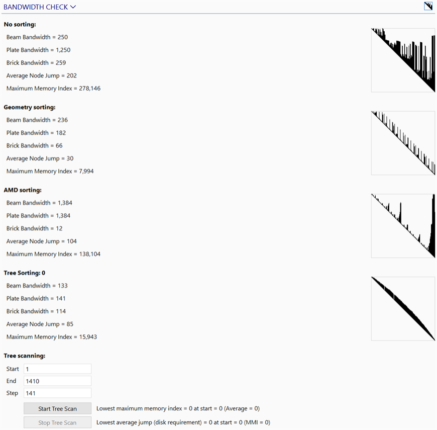
Check bandwidth
Checks and visualises the effects of different bandwidth minimisation (i.e., node ordering) strategies. This is mainly useful when using the Skyline scheme because for the Sparse scheme AMD is almost always the best, and for the Iterative (PCG) scheme the node ordering is not important in terms of storage requirements.
The matrix shapes are displayed together with statistics. The best method to use depends firstly on the amount of physical memory (RAM) available and secondly on the amount of disk space. If a large amount of RAM is available, it is preferable to reduce the Average Node Jump (which corresponds to the time spent reading and writing to disk), otherwise it is preferable to reduce the Maximum Memory Index (which corresponds to RAM requirement).
The optimum RAM needed and the amount actually used are reported in the solver log file. If the amount of RAM needed is less than or equal to that actually used, the solver can run with good performance. If the first amount of RAM needed is greater than that actually used, the solution time can increase significantly.
Tree scanning
Defines the range and interval of the tree scan for the purpose of finding an optimal starting node. For example 1,100,10 will check every tenth node, starting at node 1 (i.e., 1, 11, 21, ...).
-
Start
The starting node number of the scan, typically node 1.
-
End
The ending node number of the scan, typically the last node number of the model.
-
Step
The size of the scanning interval.
-
Start Tree Scan
This commences the tree scan procedure.
-
Stop Tree Scan
Stops the tree scan procedure at the end of the current scan.
Beam/Plate/Brick Bandwidth
The maximum node number difference between any two connected nodes amongst each respective entity type.
Average Node Jump (Disk requirement)
The average bandwidth of the entire matrix, which corresponds to the time spent reading and writing to disk.
Maximum Memory Index (MMI / RAM requirement)
An indicator that corresponds to the RAM requirement for the node ordering schemes.
See Also