Special Topics: Solver Bandwidth Minimisation

Description

Finite element analysis involves the assembly and solution of a matrix defining the relationship between force and displacement (i.e., the stiffness matrix). Finite element stiffness matrices are generally symmetric and, with appropriate ordering of the nodes, banded.

Symmetric means that the upper triangle of the matrix is a mirror image of the lower triangle (or numerically that the transpose of the stiffness matrix is the same as the stiffness matrix itself).

Banded means that the non-zero entries are clustered together near the diagonal of the matrix; the height of each column is called the bandwidth. This bandwidth is directly related to the maximum node number difference across any element together with the number of degrees of freedom in the element (e.g., a beam element connected to nodes 23 and 65 in a mesh, will produce a bandwidth of (65 - 23 + 1) × 6 = 258, while a beam connected to nodes 23 and 24 will produce a bandwidth of only 12).

Strand7 offers two direct solver technologies (a skyline solver and a sparse solver) and one iterative solver (a preconditioned conjugate gradient solver). The direct solvers use a technique known as factorisation to convert the matrix to a form that allows an efficient solution (this is similar to Gaussian elimination). The iterative solver does not factorise the matrix.

Solver Scheme

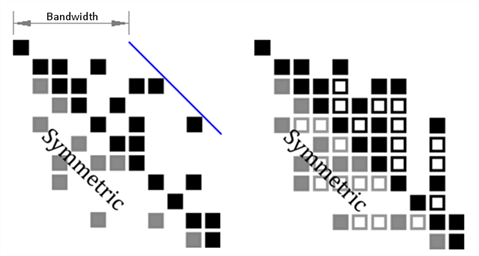
An example stiffness matrix is shown below on the left and its skyline representation is on the right where:

solid black squares represent initial non-zero entries;
hollow black squares represent stored zeros; they are stored because they are expected to become non-zero during the factorisation process;
grey squares represent implicit symmetrical entries, which are not stored;
white space represents zero entries not stored.

Skyline Solver

For the skyline solver, the average bandwidth times the number of equations gives the storage requirements for the stiffness matrix; the maximum bandwidth has a major impact on the amount of RAM required.

While the number of equations is fixed for any given model, the bandwidth can be minimised by reordering the node numbers. The skyline solver stores columns from the stiffness matrix, from the highest non-zero entry down to the diagonal. For highly banded, dense matrices, the scheme is efficient; however, if the matrix is not well banded, excessive memory and time can be spent storing and manipulating zero entries.

To improve the performance of the skyline solver, Strand7 includes two methods of minimising the bandwidth: the geometry and tree methods.

Examples of meshes which typically perform well under the skyline solver are regular brick meshes.

Direct Sparse Solver

The Strand7 sparse solver is a high performance option that is useful for large models. Sparse solvers allow a fast solution of large systems of equations by exploiting the so-called sparsity of the matrix. A matrix is sparse if the number of non-zero entries is small compared with the total number of entries in the matrix. Plate meshes with complex topology can be expected to solve more than an order of magnitude faster using the direct sparse solver compared with the skyline solver. Compared with the skyline solver, the sparse solver will almost always require less storage to store the stiffness matrix. However, in some cases, the sparse solver may require more RAM than the skyline solver.

Iterative Preconditioned Conjugate Gradient Solver (PCG)

Unlike the skyline and sparse solver schemes, the preconditioned conjugate gradient scheme uses an iterative approach to converge on the solution to the linear system without factorising the stiffness matrix. Since the scheme is iterative it is not guaranteed to converge and therefore it may fail in situations where a direct scheme succeeds. In addition, singularity in models is much harder to detect with the iterative solvers since there is no division involved in the process (as is the case with factorisation where each equation is divided by the diagonal entry of the matrix - a zero diagonal usually means a zero stiffness).

Because the stiffness matrix is never factorised by the PCG solver, it requires less storage compared with direct schemes. This is because none of the zeros in the matrix are stored or acted upon. The matrix is stored in compact form. However, for the PCG solver to be efficient, all of the compact matrix needs to be in RAM. If this is not the case, the solver will still run, but it will take significantly longer since it needs to continually swap the matrix to disk at every iteration.

The PCG solver typically performs best on brick meshes.

Node Ordering

Approximate Minimum Degree (AMD)

If the sparse solver is used, node ordering should always be set to AMD. Whilst the sparse solver scheme aims to store only non-zero matrix entries, some of the zeros will become non-zero during the factorisation stage. The sparse solver therefore needs to allow space for these so-called fill-ins. The AMD node ordering attempts to minimise the fill-in.

Geometry Method

The Geometry method is applicable to the skyline solver and considers the geometric proximity of nodes with respect to their neighbours. Although geometric proximity has no strict relevance to bandwidth since bandwidth depends only on connectivity (i.e., topology), in practice, when two nodes are geometrically close by they are likely to be more closely connected than two nodes that are very far from each other. Therefore it makes sense to try and reduce the node number difference between nodes that are geometrically close to each other. The geometry sorting method performs a 3-dimensional sort of the nodes based on their coordinates. It will firstly order the nodes in increasing X, Y or Z ordinate depending on which axis forms the shortest distance of the model dimensions. It then performs a second ordering based on the axis with the second shortest distance. Finally it orders according to the remaining axis (i.e., in the longest direction).

This algorithm performs well on structures that are regular or that have a dominant length dimension in one of the global coordinate axes directions (e.g., squares, cubes and rectangular meshes).

Tree Method

The tree method is applicable to the skyline solver and considers only the connectivity of adjacent elements. This method is based on a binary tree definition of the element connections. It performs well in the majority of cases and better than the geometry method in an average sense, although in many particular cases, geometry sort will be better. The tree start parameter defines the starting point of the tree structure by entering a node number. Different starting points will produce different orderings and therefore different bandwidths.

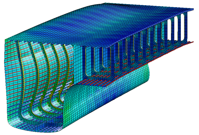
Performance figures for the algorithms on the example mesh shown below are presented in the following table. Times measured on an Intel® Core™ i7-4790K Processor.

Solver	Node ordering	CPU time (seconds)	Stiffness [K] matrix sIze (MB)	RAM needed (MB)
Sparse	AMD	2.547	134.9	36.8 Optimum
Skyline	Geometry	56.391	853.0	68.4 Minimum
Skyline	Tree (Lowest Average Jump)	49.828	764.3	45.5 Minimum
Skyline	Tree (Lowest MMI)	53.578	790.7	29.1 Minimum

The example catamaran compartment mesh consists of 14808 nodes, 5630 beams and 14529 Quad4 plates. The stiffness matrix consists of 86082 equations.

Bandwidth Minimisation

Neither geometry nor tree methods are optimal for all models using the skyline solver. For large models both methods should be investigated to find the best option. Furthermore, various points on the model should be checked using the tree method, or alternatively the automatic tree scan option can be run to systematically check different starting nodes; the tool records the best one found. Different models are suited to different bandwidth minimisation strategies. Generally models that have a dominant length direction in the X, Y or Z axis are suited to the geometry method. Most other models are suited to the tree method. Models where the geometry "branches" off in all directions are also suited to the tree method.

The SOLVERS: Matrix page provides a means for visualizing the actual shape of the global stiffness matrix. This can be used to make an informed decision about the method to use. The best method to use depends firstly on the amount of physical random access memory (RAM) available on the system, and secondly on the amount of disk space to store the matrix. On a system with a "large" amount of RAM, the aim should be to reduce the Average Node Jump; on a system with a smaller amount of RAM, the aim should be to reduce the Maximum Memory Index. The average node jump is proportional to the average bandwidth reported in the solver log file (the solver effectively reports the average node jump multiplied by the number of degrees of freedom per node, so in most 3D beam and plate/shell problems, the solver value will be approximately six times the average node jump, or three times the average node jump for brick models). The Maximum Memory Index corresponds to RAM requirement and, consequently, the need to use the hard disk as virtual memory.

The solver logs the minimum RAM needed and the amount actually used. If the amount used is greater than the amount required, the solver will provide good performance. Otherwise solution time can increase significantly.

The shape of the matrix and the size of the bandwidth are dictated by the type of element in the model and the node numbering sequence.

The following table summarises the bandwidth for a number of different element types.

Element type	Bandwidth for one element
Truss in 3D	6
Beam in 3D	12
4-node Plane Stress	8
4-node Plate/Shell	24
8-node Curved Shell	48
9-node Curved Shell	54
Tetra4 Brick	12
Tetra10 Brick	30
Tetra20 Brick	60

Elements with more nodes and degrees of freedom have larger bandwidths. For example 3D problems (such as shell problems) generate matrices with larger bandwidths than 2D problems (such as plane stress problems).

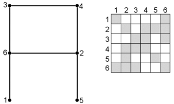
The node numbering sequence has the most significant effect on the skyline matrix size. The bandwidth of the matrix is determined by the maximum difference between any two connected nodes in the finite element model. To minimise the bandwidth the nodes should be ordered in a manner that reduces the maximum difference. The following figures illustrate the effect of node numbering on the bandwidth of the stiffness matrix. For simplicity, in the figures it has been assumed that each node has one degree of freedom.

With the scheme below, the maximum node jump is 5 (nodes 1 and 6).

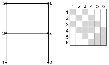
With the scheme below, the maximum node jump is 2 (nodes 1 and 3).

To reduce the solution time and storage requirements for a given model, it is necessary to reduce both the maximum and the average bandwidths. The average bandwidth (together with the total number of equations) is a direct indicator of the total storage requirement (and number of numeric operations required). The maximum bandwidth affects the maximum memory index calculation and hence the amount of memory (RAM) required to solve the matrix, as illustrated in the figure below. It is a measure of the effective area of the triangle (shown in the following figure) in terms of nodes (not taking into account the number of degrees of freedom per node).

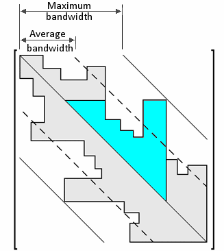
For a fast solution of the matrix, the minimum section of the matrix that should be stored in RAM corresponds to the cyan triangular section of the matrix shown in the figure. This triangle changes in size depending on the equation being reduced.

The re-ordering process only renumbers the node numbers internally for the solver. The real numbers of the nodes and elements remain unaffected. The results calculated internally in the re-ordered numbering system are mapped back to the user-specified numbers for output.