Results Interpretation: Fast Fourier Transform
Description
FFT (Fast Fourier Transform) is an algorithm for obtaining the frequency components of a time signal.
A periodic signal in the time domain can be decomposed, by Fourier analysis (Fourier series), into a sum of sine (or cosine) waves of different frequencies, starting at the fundamental frequency and followed by multiples of the fundamental frequency. The fundamental frequency of the decomposed time domain signal is equal to the inverse of its entire time period
. If the amplitudes of the sine signals are plotted against their frequencies, a spectrum is obtained in the frequency domain. This spectrum reveals information about the frequency content of the time domain signal. The transform from the time domain into the frequency domain and its inverse transform (i.e., from the frequency domain back to the time domain), form a Fourier transform pair.
When the time period of the time domain signal approaches infinity, the Fourier transform pair is turned into an integral transform pair and the function in the frequency domain becomes a continuous function of frequency. When the process is dealt with by computers (i.e., doing the transform numerically), the functions need to be sampled. In this case, the continuous Fourier transform pair becomes the Discrete Fourier Transform (DFT) pair, expressed by
-
Forward Transform:
-
Inverse Transform:
where is the number of sampling points and
is the imaginary unit. FFT is simply a fast algorithm for calculating the above transform by letting
be a power of 2 (e.g., 64, 128, 512, ...) and using the resulting characteristics involved in the calculation.
In Strand7,the FFT function is available for Results Graphs: 2D Graph Tab.
The FFT output can be configured under Graph Options: FFT Options.
Relationships between Parameters
The relationships between parameters involved in an FFT analysis are briefly summarised in the following.
- The interval between samples is
.
- The frequency resolution (or the frequency of the first harmonic component) is
. This means that the frequency resolution increases as the sampling length of the results graph increases.
- The sampling frequency is
.
- The Nyquist frequency is
which is related to aliasing.
More details are available in the Strand7 Theoretical Manual.
Example
A spring modelled with a single Beam Properties: Spring-Damper element is fixed at one end; at the other end a unit enforced displacement is applied.
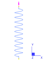
The enforced displacement varies as a function of time described by a Factor vs Time LAYOUTS: Tables representing the following equation (i.e., a signal of 0.5 Hz and 2.5 Hz with amplitudes 3.0 mm and 2.0 mm respectively).
A full system SOLVERS: Linear Transient Dynamic Settings is run with 500 steps of 0.02 s.
After solving, the time history of displacement is plotted to confirm that the output matches the input table:
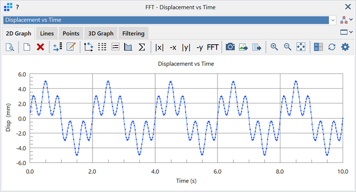
As this result is composed of two inputs with distinct frequencies and amplitudes, we expect to recover the components via the FFT Magnitude result. The figure below shows this result for a None filter window without Divide by N. This is an FFT plot that is consistent with the forward transform - backward transform definition given above; that is, in the forward transform, the division by N is not performed, whereas in the backward transform, this division is performed.
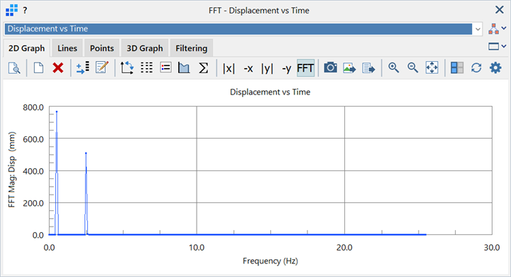
In this example, 500 time steps are used. For the FFT calculation, Strand7 automatically expands this to 512 points by fitting piecewise polynomials (of order 2 in this case) through the available points, and then evaluating 512 equi-spaced points through these polynomials. 512 is the next highest power of 2 for the time steps available (29 = 512); the piecewise polynomial interpolation function can be set from order 2 to 6. The re-sample time step is now T/N = 10/512 = 0.01953 s instead of 0.02 s. The frequency will range from 0.0 Hz to the Nyquist frequency, 1/(2D) = 1/(2x0.01953) = 25.6 Hz, at a frequency step of 1/T = 1/10 = 0.1 Hz. The FFT result is then presented via 256 points; only one half (the positive half) of the transformed series is used, which is the value of N used by the Divide by N option.
To help generate FFT results that are more meaningful from an engineering perspective, the Divide by N option may be set. Re-plotting the FFT above with this option gives the following result:
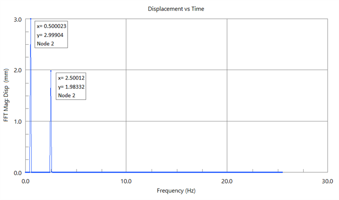
This graph illustrates that a 2.999 displacement amplitude is contributed by an input with a frequency of 0.5Hz and that a 1.983 displacement is contributed by an input with a frequency of 2.5Hz. These coincide with the applied Factor vs Time table magnitudes of 3.0 and 2.0, respectively.
In most practical situations, where the response is a result of many input frequencies, the inputs are not as clearly defined as the simple example above.
Quite often, the spike is composed of multiple points. This can be either due to the choice of filter window or simply due to the interaction of multiple inputs at close frequencies. The figure below shows the same FFT plot using the Hann filter window:
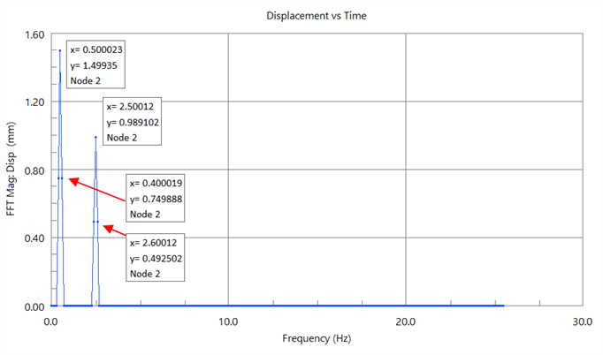
This FFT plot shows that now the first spike is composed of three points, one with amplitude of 1.499 at 0.5 Hz and two others close to 0.5 Hz with amplitude of around 0.749. Summing these three values gives an amplitude of 2.999, which is close to the expected value of 3.0. Similarly, the three values that comprise the second spike sum to 1.976, which is close to the expected value of 2.0. This result can be taken to mean that either there are three distinct frequency inputs contributing to the spike, or that the input frequency is smeared over a frequency range that is larger than the frequency resolution defined above. If it is the latter, then the summation of the three amplitudes is valid. If it is the former, the summation may not be valid as it does not take into account the phase relationship between the three input frequencies.
[1] Press, W.H. 1992, Numerical Recipes in Fortran 77-The Art of Scientific Computing, 2nd edn, Cambridge University Press.
See Also