SOLVERS Load: Nonlinear Static
Unstaged analysis
Staged analysis
Description
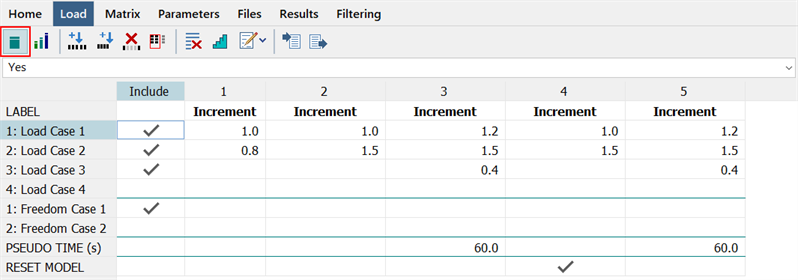
Selects the load and freedom cases to include in the analysis and assigns load factors.
Each increment or load step (i.e., column), represents a load combination and corresponds to a result case in the results file. The values entered in the grid are scaling factors for each load and freedom case. Factors can be positive, negative or zero.
Each column in the grid represents the total load applied at that increment as a linear combination of the included load cases based on the factors entered. The factors do not represent the difference in the load from the previous column. For example, a column full of zeros means that all load is removed, not that none is added. This table is therefore conceptually equivalent to the linear load case combinations table used in linear static analysis (see CASES: Combination Cases).
If a case is excluded (i.e., not checked), it makes no contribution to the solution irrespective of the load factors specified.
Factors can also be applied to scale the freedom cases. However, these only have an effect if the freedom case includes non-zero enforced restraints. In that case, the factors scale those enforced restraint values enabling the simulation of varying enforced displacements from increment to increment (see Node Attributes: Restraint for more information about enforced displacements). In addition, a zero factor applied to an included freedom case does not remove the restraints, it just scales the enforced displacements of that freedom case to zero. If a restraint is already assigned as a zero enforced restraint, the load factor has not effect.
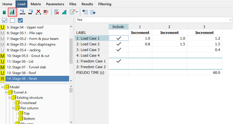
Stages List and Group Tree Preview
In staged analysis, there is one set of load factors (i.e., one grid) for each stage. The current grid always refers to the highlighted stage in the stages list.
Stages can be activated or deactivated for analysis by clicking the yellow square to toggle its state from active (yellow) to inactive (white). Squares are marked with the letters M, U, or R depending on whether they are Morphed stages, Unmorphed stages or Reset stages. This stage setting cannot be changed here; it is assigned and changed via Global: Stages.
The group tree preview shows the active groups for the highlighted stage. This information is given only for reference as the stage definitions cannot be edited here. Stage definitions are edited via Global: Stages.
Selections
Selects all stages, clears all stages, or inverts the active status of all stages.
Only active stages are considered in the analysis.
Toolbar Functions
Unstaged Analysis
If set, ignores staging information and solves for a single set of increments for the entire structure (i.e., all elements are included in the analysis).
Staged Analysis
If set, the stage list and the group tree preview are shown, enabling the definition of one set of increments for each stage.
This option becomes available only if stage information is defined under Global: Stages.
Insert increment
Inserts a new increments before the highlighted cell.
New factors are linearly interpolated from the cells before and after the inserted column.
Add increment
Adds a new increments to the end of the list.
New factors are initialised with zero values.
Delete selected increments
Deletes the highlighted columns, thereby removing those increments.
Reset Increment Totals
Opens the SOLVERS Increments: Reset Increment Totals window to change the total number of increments.
Clear All Values
Sets all load and freedom case factors in the grid to zero. For a staged analysis, only the factors in the current stage are set to zero.
Auto Create Increments
Opens SOLVERS Increments: Auto-Create Increments, which enables load factors to be automatically entered in the grid for either constant or linear variations between increments. The tool can operate on the current grid or on multiple grids in a staged analysis.
Auto Rename Increments
-
Rename Increments
Resets the increment names to the default "Increment 1", "Increment 2", and so on.
-
Renumber Increments
Resets the increment names to numerical labels "1", "2", and so on.
Import data
Opens the Open File dialog, which enables the import of a pre-saved .LCF load case factors file into the grid.
Export data
Opens the Save File dialog, which enables the export and saving of the load case factors and combinations into an .LCF load case factors file; this can be imported into another model.
PSEUDO TIME
Pseudo time is an optional value in time units that can be assigned to increments.
If pseudo time is included and nonlinear material (MNL) is enabled, material properties that have a Factor vs Time table assigned (e.g., Modulus vs Time) are scaled according to the pseudo time value defined for the increment. The entire increment uses the same pseudo time value, irrespective of any sub-stepping that may occur.
RESET MODEL
By default, a nonlinear analysis is a sequential analysis in which the results of the previous increment become the starting point for the current increment. For example, if a beam has yielded in the previous increment due to the applied load, and in the current increment all of the load is removed, the results of the current increment will represent the unloading of the yielded beam. This will produce a result with some residual stress and displacement, even though there is no external load applied to the beam.
In the case where it is desired to treat an increment as an independent analysis, not as an analysis that follows the previous increment, the increment can be assigned the RESET MODEL option. This clears the solution history up to that point and solves the increment as if it were the first increment in the analysis (i.e., a fresh start). The next increment can itself be reset, or it can continue from the current increment, depending on its RESET MODEL option.
This option is available only for unstaged analysis. In staged analysis, a similar functionality can be applied by using the Reset Stage type (see Global: Stages).
Right-click Functions
Right-clicking the spreadsheet area opens a popup menu and provides additional functions. See Strand7 Interface: Right-click Functions.
See Also