Solvers Overview: Linear Buckling

Description

The Linear Buckling solver calculates the buckling load factors and corresponding mode shapes for a structure under given loading conditions. It is based on the assumptions that there exists a bifurcation point where the primary and secondary loading paths intersect, and before this point is reached, all element stresses change proportionally with the load factor (i.e., the response is linear and elastic up to the bifurcation point).

The solver can be executed in two run modes.

1. Variable Case

The first run mode involves the calculation of the buckling load factors based on a single variable load case whose results are available as a result case in a linear static, nonlinear static or quasi-static result file. The linear buckling solution is obtained by solving the following eigenvalue problem:

where

= global stiffness matrix,

= global geometric stiffness matrix produced by the results in the variable result case,

= buckling load factor (scaling factor on the load in the variable case to cause buckling), and

= buckling mode vectors (buckled shape).

2. Variable Case + Constant Case

The second run mode involves the calculation of the buckling load factors based on a single variable load case and a single constant load case. The results of both cases must be available as result cases in a linear static, nonlinear static or quasi-static result file. The linear buckling solution is obtained by solving the following eigenvalue problem:

where

= global stiffness matrix,

= global geometric stiffness matrix produced by the results in the variable result case,

= global geometric stiffness matrix produced by the results in the constant result case,

= buckling load factor (scaling factor on the load in the variable to cause buckling with the load in the constant case fully applied), and

= buckling mode vectors (buckled shape).

Global Stiffness Matrix

The global stiffness matrix will depend on the initial conditions used, and will take into account the following:

If the initial condition result case considers geometric nonlinearity, the tangent stiffness assembled in the geometric nonlinear analysis will be used as the global stiffness matrix; this requires the addition of a geometric stiffness matrix, [KG], to the elastic stiffness matrix.
If the initial condition result case considers contact between two or more bodies, or compression-only supports, the tangent stiffness will take this into account; inactive contact elements, cutoff bars and supports in the initial condition result case are inactive in the linear buckling analysis.
If the initial condition result case considers nonlinear material behaviour, the tangent stiffness due to material nonlinearity is also considered in the linear buckling analysis.

Irrespective of the initial conditions used, the global stiffness matrix used by the linear buckling solver remains constant. That is, the solution is still a linear buckling solution, not a nonlinear buckling/post-buckling solution.

Geometric Stiffness Matrix

The geometric stiffness matrix, also known as the initial stress stiffness matrix, is a symmetric matrix that accounts for the element stress due to the applied load. The matrix can optionally also account for changes in tangent stiffness associated with so called "follower" loads; these are distributed loads that change direction as the structure deforms. An example of this type of load is a normal pressure on a plate element, which always follows the normal surface direction of the plate.

The buckling solution requires a previously calculated static solution, which is used as initial conditions to determine the stress state of the structure (i.e., to calculate the geometric stiffness matrix). The initial solution can be a result case from the SOLVERS: Linear Static Settings, SOLVERS: Nonlinear Static Settingsand SOLVERS: Quasi-static Settings. If the initial solution comes from the Linear Static solver, CASES: Combination Cases may also be used as initial conditions. If the initial solution comes from the Quasi-static or Nonlinear Static solver, the restart file (SOLVERS: Files) for that particular solution is needed by the Linear Buckling solver, so the option to save the restart file must be set before running the initial solution (see Special Topics: Solution Restart).

Procedure

The Linear Buckling solver executes the following steps:

Calculates and assembles the global stiffness and geometric stiffness matrices. In the stiffness calculation, material temperature dependency is considered through the user nominated temperature case (see Special Topics: Temperature Dependence). Constraints and links are assembled in this process. However, the constant terms for enforced displacements, shrink links and multi-point links are ignored, and the restraints are treated as fixed restraints.

The geometric stiffness matrix is assembled based on the stress state of the structure calculated in the initial file. If the initial file is from a nonlinear analysis, the stiffness matrix calculation is based on the material status and geometry as calculated in the initial analysis. In other words, a yield modulus will be used if the material has yielded and the deformed geometry will be used if the initial solution included nonlinear geometry. In addition, the active/inactive state of point contacts, cutoff bars and compression-only element supports will be considered when assembling these in the stiffness matrix of the linear buckling analysis (the stiffness matrix will maintain their state in the nonlinear solution file).

In calculating stresses for the geometric stiffness matrix, the solver includes thermal strains and other pre-loads applied in the initial solution.

If the effect of follower loads is requested, the geometric stiffness matrix is augmented to account for these.
Modifies the stiffness matrix when a shift value is applied. This allows for the calculation of higher order modes if required.
Solves the eigenvalue problem to get buckling load factors and the corresponding buckling modes using the Sub-Space Iteration method.

Notes

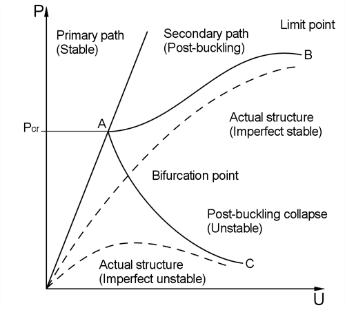
The linear buckling analysis assumes the existence of a bifurcation point where the primary and secondary loading paths intersect (point A in the figure below). At this point, more than one equilibrium position is possible. The primary path is not usually followed after loading exceeds this point and the structure is in the post-buckled state. The slope of the secondary path at the bifurcation point determines the nature of the post-buckling. A positive slope indicates that the structure will have post-buckling strength whilst a negative slope means that the structure will snap through or simply collapse. Real structures have geometric and loading imperfections, often causing the primary path curve and the bifurcation point to disappear.
The linear buckling analysis assumes that the stresses in the structure increase proportionally with the load. When the deformation is large enough to disturb the stress distribution, linear buckling results will no longer be valid. In this case, a nonlinear solution is more appropriate for a realistic prediction of the structure's capacity.
There are many factors in real structures that have a large influence on the stability and critical buckling load. The linear bifurcation analysis neglects all of these and assumes that the structure is perfect.
For real structures linear buckling analysis is best used for preliminary design and for studying the effects of various parameters. When the above assumptions are fully or nearly satisfied, linear buckling analysis will give accurate answers. If a more accurate estimate of the buckling load is required, it is recommended that a nonlinear analysis be carried out so that the effect of pre-buckling deformation can be included and the post-buckling capacity predicted.
Negative modes calculated by the Linear Buckling solver indicate that buckling will occur if the load is reversed. To avoid the calculation of negative modes, a positive shift value can be used to calculate higher (more positive) modes (a zero shift means that modes near zero, above and below, are calculated).