Beam Elements: Nonlinear Material Beams

Description

Nonlinear material beams can be modelled using one of three methods in Strand7:

The first method requires the definition and selection of moment-curvature tables for the two principal planes of the beam, together with a stress-strain table for the axial direction. For this method, the moment-curvature and axial stress-strain components are considered independently (i.e., yielding in one axis does not affect the other axes). The method is a simplified one, applicable when only one axis dominates the response.
The second method uses a single stress-strain table in conjunction with the definition of the cross section geometry to consider the combined nonlinear axial and bending behaviour of every beam fibre in the cross section. The beam element is discretised over the cross section to define a number of stress sampling points. Based on the section shape and the axial force and moments in the beam, the fibre stress/strain pairs are calculated at each sampling point, and the iterative plasticity algorithm ensures that these stress/strain pairs satisfy the stress-strain table (i.e., the material constitutive relationship). This is repeated at a number of stations, or integration points, along the element length to produce section matrices at each station. The station results are numerically integrated to form the element stiffness matrix. This method offers the possibility of simulating complex nonlinear material behaviour of beams including force-moment coupling between the three axes.
The third method uses a single stress-strain table with the von Mises or Tresca yield criterion. This method has the same requirements at method 2 in terms of the cross section definition and discretisation. However, in addition to fibre stress due to axial force and bending moments, it also considers shear stresses due to torque and transverse shear force. With these stresses it is possible to evaluate a von Mises or Tresca stress to use for the respective yield criteria. This method offers the possibility of simulating complex nonlinear material behaviour of beams including force-moment coupling between the three axes, taking into account transverse shear stress contribution to yield stress.

How to use nonlinear material beams

The following summarises the procedure to set up nonlinear material beam elements for either method 2 or method 3.

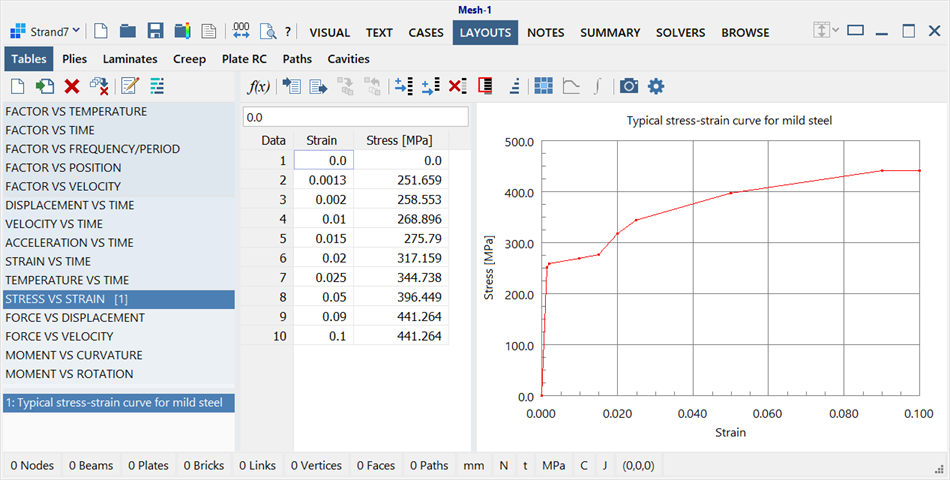
Firstly a Stress vs Strain table for the material is defined via LAYOUTS: Tables.

Data can be entered directly into the table, imported from a file, copied/pasted from the clipboard, or generated using the Equation editor.

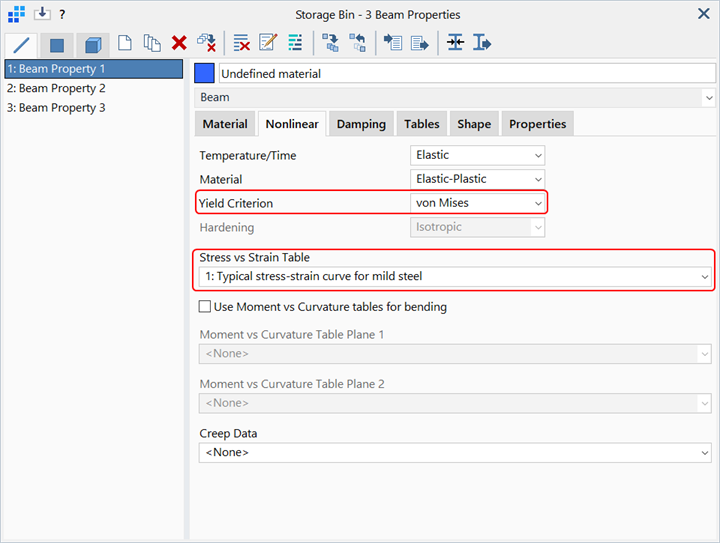
The Stress vs Strain table is then assigned to the beam property by using Assign to property in LAYOUTS: Tables. Alternatively, it can be selected or changed later via the Common Properties: Nonlinear tab of Global: Beam Properties; the required Stress vs Strain table is selected from the Stress vs Strain Table dropdown list.

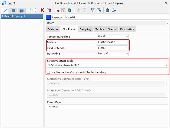
For analysis using methods 2 or 3, the option Use Moment vs Curvature tables for bending must be cleared. This then enables the selection of Fibre, von Mises or Tresca under Yield Criterion.

To use method 1, the option Use Moment vs Curvature tables for bending is set; this then changes the label to Axial Stress vs Strain Table and two Moment vs Curvature tables may be selected.

Under the Common Properties: Sections tab, the number of Integration Points for the beam can be set. Integration Points are the sampling points along the length of the beam at which the section matrices are calculated based on the axial force, the moments, the section shape and the stress-strain or moment-curvature relationships selected. These are then integrated to produce the stiffness matrix for the element. The default setting is 5, which should be sufficient for the majority of cases.

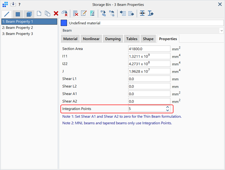
Integration Points also controls the number of integration points used to calculate the stiffness matrix for tapered beams, irrespective of whether the material is linear or not.

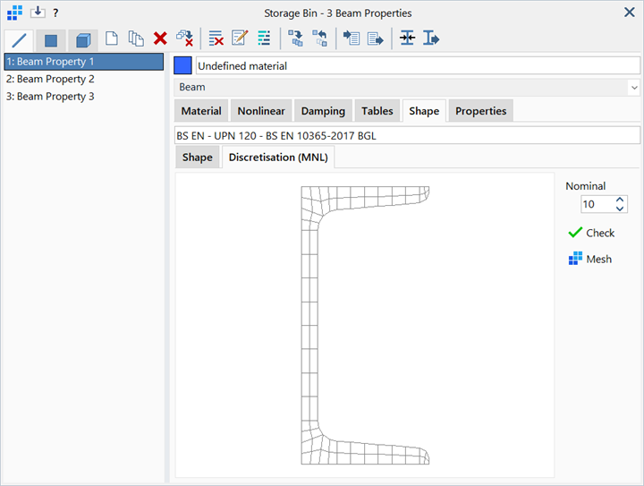
The discretisation of the beam cross section can be specified for different beam cross section geometries via Properties: Beam Cross Section Shape on the Discretisation (MNL) page.

The following options are available depending on the beam cross section type:

Solid and hollow circle

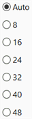
For circular cross sections the number of Circumferential Divisions is set. When Auto is used, the number of divisions in both the circumferential and radial directions are automatically determined to produce approximately square cells based on the radius to wall thickness ratio. Alternatively the number of divisions can be set from 8 to 48, in multiples of 8.

BXS and BGL

For BXS cross sections, the number of divisions used for the analysis is at least as many as the number of elements in the original mesh. If a coarse mesh was used to construct the BXS, Nominal Divisions can be used to further subdivide the mesh.

BSL and other standard shapes

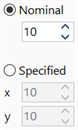
For these cross sections, Nominal Divisions sets the number of divisions in the x and y directions. The value is taken as the number of divisions along the longest edge of the section, with the number of divisions in the other direction being approximately proportional to the length ratios.

If Specified Divisions is set, the number of divisions in the x and y directions can be set independently.

See Properties: Beam Cross Section Shape.

When the number of integration points or divisions of the cross section is increased, the result will usually be more accurate but the solution time will increase.

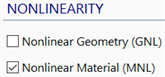
After the beam property has been defined, the Nonlinear Material (MNL) solver option in SOLVERS Home: Nonlinearity must be set to consider the material nonlinearity (i.e., the stress-strain table). The MNL option is available for SOLVERS: Nonlinear Static Settings, SOLVERS: Nonlinear Transient Dynamic Settings and SOLVERS: Quasi-static Settings depending on the analysis required.

Solver parameter that control iteration and hence convergence can be adjusted in SOLVERS Parameters: ITERATION (Structural). For example, the NONLINEAR MATERIAL MODULUS UPDATE slider controls the update of the local stiffness matrix for nonlinear material problems. The slider sets the ratio of tangent modulus to secant (or initial) modulus used in the stiffness matrix. The Stable solution (i.e., ratio = 0.0), uses the secant modulus; the Fast solution (i.e., ratio = 1.0), uses the tangent modulus (approximately). At Fast, the solution will converge in fewer iterations but the solution may not be numerically stable in some cases; a Stable solution will require more iterations but usually it is numerically more stable. The default setting is 0.5 to provide a proportion of both the secant and tangent modulus in the formation of the stiffness matrix.

When viewing the results for a nonlinear material beam analysis there are a few points that should be noted.

While the beam is still in the elastic range all stresses can be extracted.
When the beam has yielded it is not possible to view Bending Stress results as these are no longer given by (see Results Interpretation: Result Quantities). Elements that have yielded are shown in wireframe when this stress option is requested.
When a beam has yielded, the axial stress contour may still be shown; this is calculated simply as the axial force in the beam divided by its cross section area (i.e., the average axial stress).
Fibre stresses, von Mises and Tresca stresses, which are calculated by the solver, may be contoured even if the beam has yielded. These are the stresses used by the solver to refer to the Stress vs Strain table (i.e., the yield criteria). To store these stress results so that they are available for post-processing, the Beam Fibre Results (MNL and CNL) option must be set in SOLVERS: Results before running the solver.

Stress contours after some elements have yielded
Bending Stress
Fibre Stress
von Mises Stress

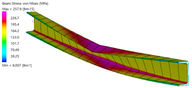
Example

The following illustrates a simple example of the plastic hinge formation in a simply-supported beam using method 2.

Description

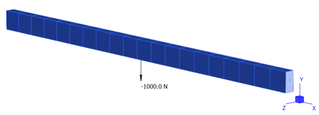
The simply supported beam is 1 m long with a rectangular cross section 50 mm × 25 mm. A central point force of FY = -1000 N is applied.

Model definition

The Stress vs Strain table is automatically defined via the three-parameter option offered by the equation editor in LAYOUTS: Tables.

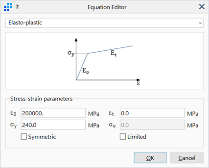
The table is assigned to the beam property and the Fibre option is selected as the Yield Criterion.

Analysis

The Nonlinear Static solver is executed with both the Nonlinear Geometry (GNL) and Nonlinear Material (MNL) options set under SOLVERS Home: Nonlinearity.

The total load is applied in one load step (SOLVERS: Load (Nonlinear Static)) together with the Displacement control (arc length) option in SOLVERS Parameters: SUB-STEPPING (Static). This enables the solver to automatically set the load steps based on the resolution of the displacement history requested. The Save sub-steps option needs to be set to obtain the load-displacement history.

Results

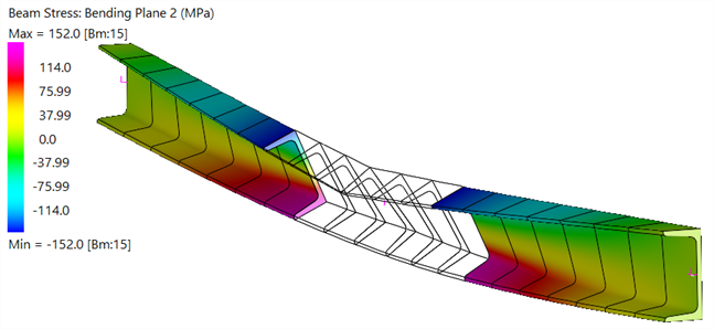
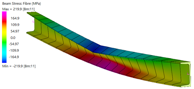
At the completion of the analysis, after clicking Solve, the results file is opened (Strand7 Menu: Results Open/Close) to inspect the solution. A contour of the fibre stress can be produced via Results: Element Results Settings. The following image is for the last result step with all of the load applied.

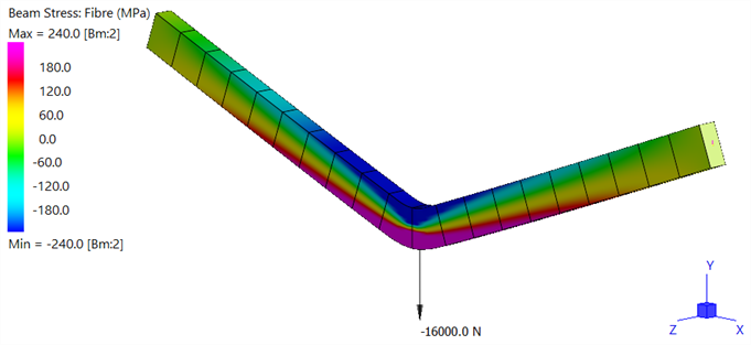
The results highlight extensive yielding in the mid-span where a plastic hinge has formed.

A detailed look at the fibre stress at a number of slices for an element at mid-span can be obtained via Results: Peek.

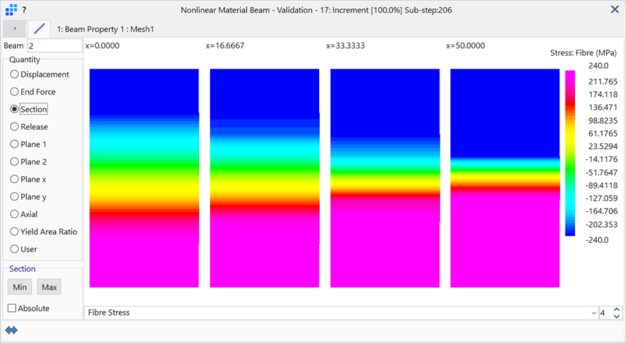
This shows the stress distribution at four equi-spaced slices along the beam length, revealing the progression of yield.

To view the force vs displacement history, a Results: Graphs is created. This is a vs Result Case graph of the DY displacement at the centre node vs Load Case/Freedom Case Factor (see New Graph: Position Tab).

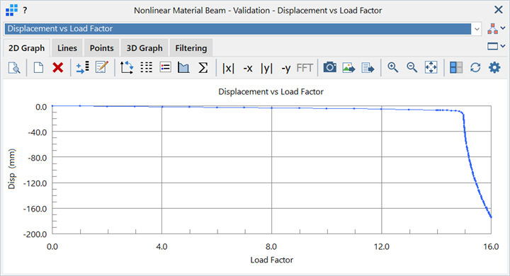
This shows that there is an approximately linear variation in displacement initially, but that at a load factor of around 14.5 (14 500 N) the structure softens and the displacement increases dramatically compared to the increase in load. This is consistent with simple calculations for the force required to just yield the outer fibres, , and the force required to produce a fully plastic section, , at the mid-span.

Since there is no post-yield modulus, the beam reaches equilibrium only because of the redistribution of bending stress into axial stress due to geometric nonlinear effects; as the hinges form, the beam becomes a two-bar linkage.